
摘要
本文将展示如何使用Python和自然语言处理构建知识图谱。
网络图是一种数学结构,用于展示可以用无向/有向图结构可视化的点之间的关系。它是一种将链接节点映射的数据库。
知识库是来自不同来源(如维基百科)的信息的统一存储库。
知识图是使用图形结构数据模型的知识库。简单来说,它是一种特定类型的网络图,显示现实世界实体、事实、概念和事件之间的定性关系。术语“知识图”最早由谷歌在2012年使用,用于介绍他们的模型。
目前,大多数公司正在构建数据湖,这是一个中央数据库,其中他们将来自不同来源的所有类型的原始数据(即结构化和非结构化数据)扔进去。因此,人们需要工具来理解所有这些不同信息的片段。知识图正在变得越来越流行,因为它们可以简化大型数据集的探索和洞察发现。换句话说,知识图连接数据和相关元数据,因此可以用于构建组织信息资产的全面表示。例如,知识图可能替代你必须浏览以找到特定信息的所有文件堆。
由于要构建“知识”,所以知识图被认为是自然语言处理领域的一部分,因为必须经过一个称为“语义丰富化”的过程。由于没有人想手动执行此任务,因此我们需要机器和NLP算法来为我们执行此任务。
我将介绍一些有用的Python代码,可以轻松应用于其他类似情况(只需复制、粘贴、运行),并逐行通过带有注释的代码,以便你可以复制此示例(下面链接到完整代码)。
我将解析维基百科并提取一页,该页将用作本教程的数据集(下面链接)。
https://en.wikipedia.org/wiki/Russo-Ukrainian_War
具体而言,我将介绍:
- 设置:使用Wikipedia-API进行网络爬虫读取包和数据。
- 使用SpaCy进行自然语言处理:句子分割、POS标记、依赖解析、NER。
- 使用Textacy提取实体及其关系。
- 使用NetworkX构建网络图。
- 使用DateParser绘制时间线图。
设置
首先,我需要导入以下库:
## for data
import pandas as pd  #1.1.5
import numpy as np  #1.21.0

## for plotting
import matplotlib.pyplot as plt  #3.3.2

## for text
import wikipediaapi  #0.5.8
import nltk  #3.8.1
import re

## for nlp
import spacy  #3.5.0
from spacy import displacy
import textacy  #0.12.0

## for graph
import networkx as nx  #3.0 (also pygraphviz==1.10)

## for timeline
import dateparser #1.1.7
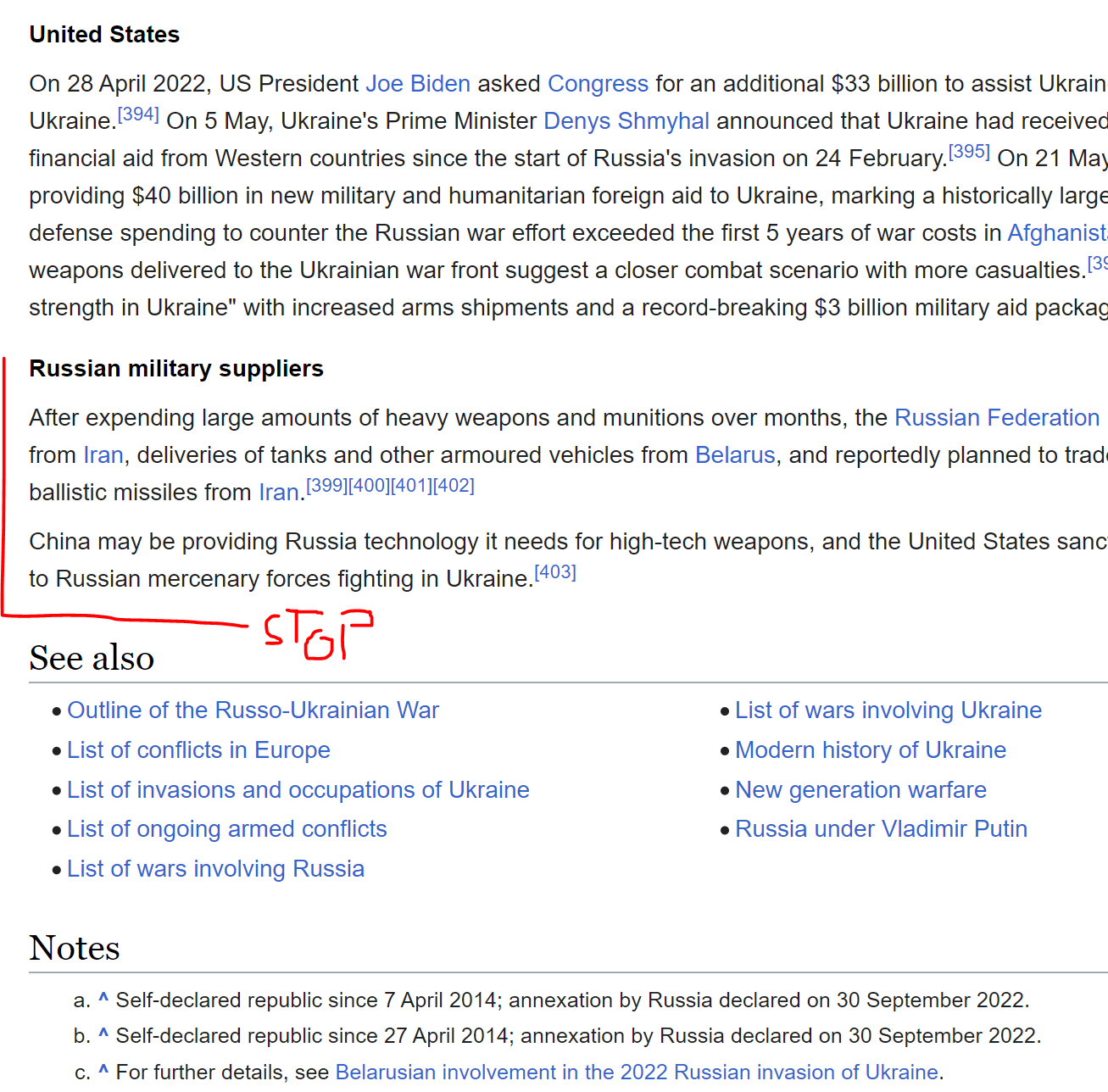
Wikipedia-api是Python包装器,可以轻松地解析维基百科页面。我将提取我想要的页面,排除底部的所有“注释”和“参考文献”:
https://miro.medium.com/v2/resize:fit:1400/1*TvUXuQI4AOyb2P9dGPDbPg.png
我们可以简单地写出页面的名称:
topic = "Russo-Ukrainian War"

wiki = wikipediaapi.Wikipedia('en')
page = wiki.page(topic)
txt = page.text[:page.text.find("See also")]
txt[0:500] + " ..."
https://miro.medium.com/v2/resize:fit:1400/1*656no9q6clzZRORjxTPp6g.png
在这个用例中,我将尝试通过识别和从文本中提取主题-动作-对象来映射历史事件(因此动作是关系)。
NLP
为了构建知识图,我们首先需要识别实体及其关系。因此,我们需要使用NLP技术处理文本数据集。
目前,这种类型任务最常用的库是SpaCy,它是一种用于高级NLP的开源软件,利用Cython(C + Python)。SpaCy使用预训练的语言模型将文本标记化并将其转换为常被称为“文档”的对象,基本上是一个包含模型预测的所有注释的类。
#python -m spacy download en_core_web_sm

nlp = spacy.load("en_core_web_sm")
doc = nlp(txt)
NLP模型的第一个输出是句子分割:决定句子何时开始和结束的问题。通常,它是通过基于标点符号拆分段落来完成的。让我们看看SpaCy将文本分成了多少句子:
# from text to a list of sentences
lst_docs = [sent for sent in doc.sents]
print("tot sentences:", len(lst_docs))
现在,对于每个句子,我们将提取实体及其关系。为了做到这一点,首先我们需要理解词性标注(POS): 标记句子中每个单词的适当语法标签的过程。以下是可能的标签的完整列表(截至今天):
- ADJ:形容词,例如big,old,green,incomprehensible,first
- ADP:介词,例如in,to,during
- ADV:副词,例如very,tomorrow,down,where,there
- AUX:助动词,例如is,has(done),will(do),should(do)
- CONJ:连词,例如and,or,but
- CCONJ:并列连词,例如and,or,but
- DET:限定词,例如a,an,the
- INTJ:感叹词,例如psst,ouch,bravo,hello
- NOUN:名词,例如girl,cat,tree,air,beauty
- NUM:数词,例如1,2017,one,seventy-seven,IV,MMXIV
- PART:小品词,例如's,not
- PRON:代词,例如I,you,he,she,myself,themselves,somebody
- PROPN:专有名词,例如Mary,John,London,NATO,HBO
- PUNCT:标点符号,例如.,(),?
- SCONJ:从属连词,例如if,while,that
- SYM:符号,例如$,%,§,©,+,-,×,÷,=,:),表情符号
- VERB:动词,例如run,runs,running,eat,ate,eating
- X:其他,例如sfpksdpsxmsa
- SPACE:空格
仅进行词性标注是不够的,模型还试图理解词对之间的关系。这个任务被称为依存句法分析(DEP)。以下是可能的标签的完整列表(截至今天):
- ACL:名词的从句修饰语
- ACOMP:形容词补语
- ADVCL:状语从句修饰语
- ADVMOD:状语修饰语
- AGENT:代理人
- AMOD:形容词修饰语
- APPOS:同位语修饰语
- ATTR:属性
- AUX:助动词
- AUXPASS:助动词(被动)
- CASE:格标记
- CC:并列连词
- CCOMP:从句补语
- COMPOUND:复合修饰语
- CONJ:连词
- CSUBJ:从句主语
- CSUBJPASS:从句主语(被动)
- DATIVE:与格
- DEP:未分类依赖项
- DET:限定词
- DOBJ:直接宾语
- EXPL:虚词
- INTJ:感叹词
- MARK:标记
- META:元修饰语
- NEG:否定修饰语
- NOUNMOD:名词修饰语
- NPMOD:名词短语作状语
- NSUBJ:名词主语
- NSUBJPASS:名词主语(被动)
- NUMMOD:数字修饰语
- OPRD:宾语谓语
- PARATAXIS:并列
- PCOMP:介词补语
- POBJ:介词宾语
- POSS:所有格修饰语
- PRECONJ:前限定词连词
- PREDET:前限定词
- PREP:介词修饰语
- PRT:小品词
- PUNCT:标点符号
- QUANTMOD:量词修饰语
- RELCL:关系从句修饰语
- ROOT:根
- XCOMP:开放从句补语让我们通过一个例子来理解词性标注和依存分析:
# take a sentence
i = 3
lst_docs[i]

让我们检查 NLP 模型预测的词性和依存关系标签:
for token in lst_docs[i]:
    print(token.text, "-->", "pos: "+token.pos_, "|", "dep: "+token.dep_, "")
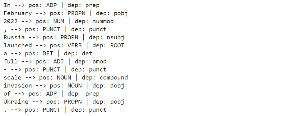
图片由作者提供
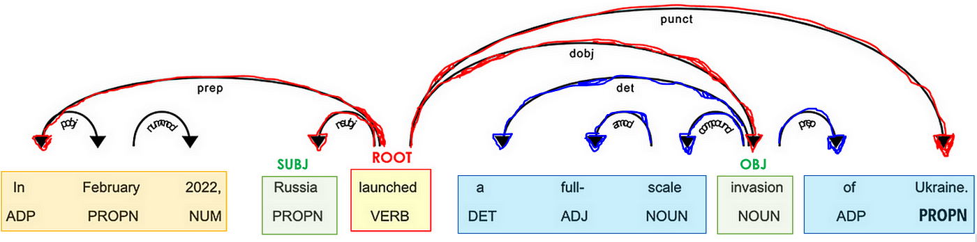
SpaCy 还提供了一个图形工具来可视化这些注释:
from spacy import displacy

displacy.render(lst_docs[i], style="dep", options={"distance":100})
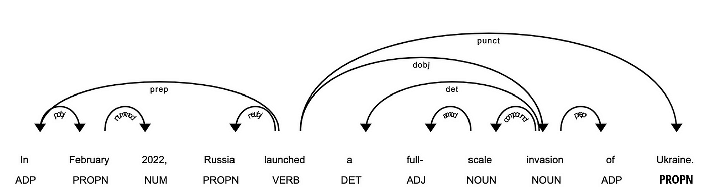
图片由作者提供
最重要的令牌是动词(POS=VERB),因为它是句子中含义的根(DEP=ROOT)。
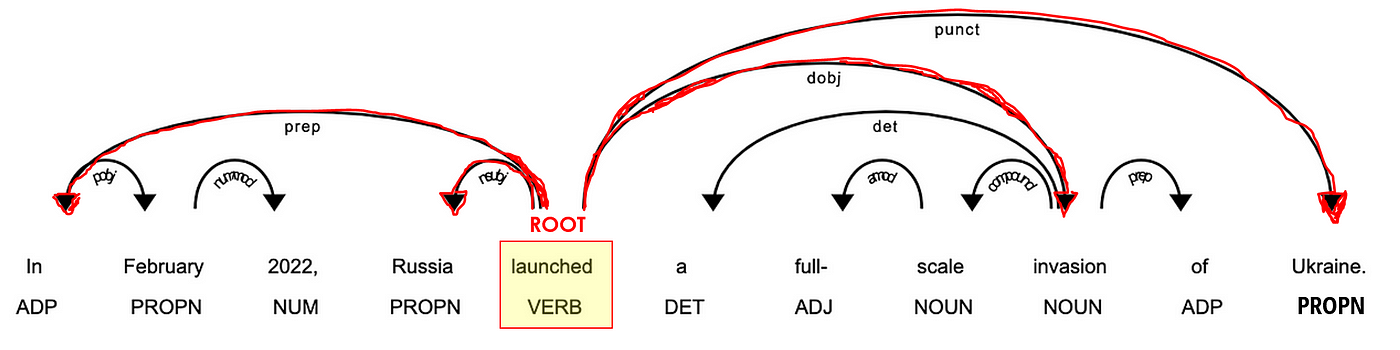
图片由作者提供
助词,如副词和介词(POS=ADV/ADP),通常作为修饰词(DEP=*mod)链接到动词,因为它们可以修改动词的含义。例如,“travel to” 和 “travel from” 尽管根是相同的(“travel”),但意义不同。

图片由作者提供
在链接到动词的单词中,必须有一些名词(POS=PROPN/NOUN)作为句子的主语和宾语(DEP=nsubj/*obj)。
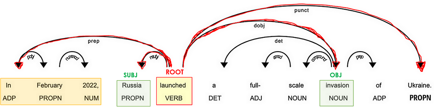
图片由作者提供
名词通常靠近作为其含义修饰符的形容词(POS=ADJ)(DEP=amod)。例如,在“good person” 和 “bad person” 中,形容词赋予名词“person”相反的含义。
图片由作者提供
SpaCy 还执行另一个很酷的任务——命名实体识别(NER)。命名实体是“现实世界对象”(即人、国家、产品、日期),“模型”可以在文档中识别各种类型。以下是可能标记的完整列表(截至今日):
- **PERSON:**人,包括虚构的人物。
- **NORP:**国籍、宗教或政治团体。
- **FAC:**建筑物、机场、高速公路、桥梁等。
- **ORG:**公司、机构、机构等。
- **GPE:**国家、城市、州。
- **LOC:**非 GPE 位置、山脉、水域等。
- **PRODUCT:**物品、车辆、食品等(不包括服务)。
- **EVENT:**命名的飓风、战斗、战争、体育赛事等。
- **WORK_OF_ART:**书籍、歌曲等的标题。
- **LAW:**命名文件成为法律。
- **LANGUAGE:**任何命名语言。
- **DATE:**绝对或相对日期或时期。
- **TIME:**小于一天的时间。
- **PERCENT:**百分比,包括“%”。
- **MONEY:**货币价值,包括单位。
- **QUANTITY:**测量,如重量或距离。
- ORDINAL:“第一”、“第二”等。
- **CARDINAL:**不属于另一类型的数字。
让我们看看我们的例子:
for tag in lst_docs[i].ents:
    print(tag.text, f"({tag.label_})")

图片由作者提供
或者更好地使用 SpaCy 图形工具:
displacy.render(lst_docs[i], style="ent")

图片由作者提供
如果我们想要向我们的知识图谱添加几个属性,这将非常有用。接下来,我们可以使用NLP模型预测的标签来提取实体和它们之间的关系。
实体与关系提取
这个想法非常简单,但实现起来可能会有些棘手。对于每个句子,我们将提取主语和宾语以及它们的修饰语、复合词和它们之间的标点符号。
这可以通过以下两种方式来完成:
- 手动,你可以从基线代码开始,该代码可能必须稍微修改并适应你特定的数据集/用例。
def extract_entities(doc):
    a, b, prev_dep, prev_txt, prefix, modifier = "", "", "", "", "", ""
    for token in doc:
        if token.dep_ != "punct":
            ## prexif --> prev_compound + compound
            if token.dep_ == "compound":
                prefix = prev_txt +" "+ token.text if prev_dep == "compound" else token.text

            ## modifier --> prev_compound + %mod
            if token.dep_.endswith("mod") == True:
                modifier = prev_txt +" "+ token.text if prev_dep == "compound" else token.text

            ## subject --> modifier + prefix + %subj
            if token.dep_.find("subj") == True:
                a = modifier +" "+ prefix + " "+ token.text
                prefix, modifier, prev_dep, prev_txt = "", "", "", ""

            ## if object --> modifier + prefix + %obj
            if token.dep_.find("obj") == True:
                b = modifier +" "+ prefix +" "+ token.text

            prev_dep, prev_txt = token.dep_, token.text

    # clean
    a = " ".join([i for i in a.split()])
    b = " ".join([i for i in b.split()])
    return (a.strip(), b.strip())

# The relation extraction requires the rule-based matching tool,
# an improved version of regular expressions on raw text.
def extract_relation(doc, nlp):
    matcher = spacy.matcher.Matcher(nlp.vocab)
    p1 = [{'DEP':'ROOT'},
          {'DEP':'prep', 'OP':"?"},
          {'DEP':'agent', 'OP':"?"},
          {'POS':'ADJ', 'OP':"?"}]
    matcher.add(key="matching_1", patterns=[p1])
    matches = matcher(doc)
    k = len(matches) - 1
    span = doc[matches[k][1]:matches[k][2]]
    return span.text
让我们在这个数据集上试一试并查看通常的示例:
## extract entities
lst_entities = [extract_entities(i) for i in lst_docs]

## example
lst_entities[i]

## extract relations
lst_relations = [extract_relation(i,nlp) for i in lst_docs]

## example
lst_relations[i]

## extract attributes (NER)
lst_attr = []
for x in lst_docs:
    attr = ""
    for tag in x.ents:
        attr = attr+tag.text if tag.label_=="DATE" else attr+""
    lst_attr.append(attr)

## example
lst_attr[i]

- 或者,你可以使用Textacy,这是一个构建在_SpaCy_之上的库,用于扩展其核心功能。这样更加用户友好,通常更加准确。
## extract entities and relations
dic = {"id":[], "text":[], "entity":[], "relation":[], "object":[]}

for n,sentence in enumerate(lst_docs):
    lst_generators = list(textacy.extract.subject_verb_object_triples(sentence))
    for sent in lst_generators:
        subj = "_".join(map(str, sent.subject))
        obj  = "_".join(map(str, sent.object))
        relation = "_".join(map(str, sent.verb))
        dic["id"].append(n)
        dic["text"].append(sentence.text)
        dic["entity"].append(subj)
        dic["object"].append(obj)
        dic["relation"].append(relation)

## create dataframe
dtf = pd.DataFrame(dic)

## example
dtf[dtf["id"]==i]

作者提供的图片
让我们也使用NER标签(即日期)提取属性:
## extract attributes
attribute = "DATE"
dic = {"id":[], "text":[], attribute:[]}

for n,sentence in enumerate(lst_docs):
    lst = list(textacy.extract.entities(sentence, include_types={attribute}))
    if len(lst) > 0:
        for attr in lst:
            dic["id"].append(n)
            dic["text"].append(sentence.text)
            dic[attribute].append(str(attr))
    else:
        dic["id"].append(n)
        dic["text"].append(sentence.text)
        dic[attribute].append(np.nan)

dtf_att = pd.DataFrame(dic)
dtf_att = dtf_att[~dtf_att[attribute].isna()]

## example
dtf_att[dtf_att["id"]==i]

作者提供的图片
现在,我们已经提取了“知识”,我们可以构建图形。
网络图
创建和操作图形网络的标准Python库是NetworkX。我们可以从整个数据集开始创建图形,但是,如果有太多节点,则可视化将会混乱:
## create full graph
G = nx.from_pandas_edgelist(dtf, source="entity", target="object",
                            edge_attr="relation",
                            create_using=nx.DiGraph())

## plot
plt.figure(figsize=(15,10))

pos = nx.spring_layout(G, k=1)
node_color = "skyblue"
edge_color = "black"

nx.draw(G, pos=pos, with_labels=True, node_color=node_color,
        edge_color=edge_color, cmap=plt.cm.Dark2,
        node_size=2000, connectionstyle='arc3,rad=0.1')

nx.draw_networkx_edge_labels(G, pos=pos, label_pos=0.5,
                         edge_labels=nx.get_edge_attributes(G,'relation'),
                         font_size=12, font_color='black', alpha=0.6)
plt.show()
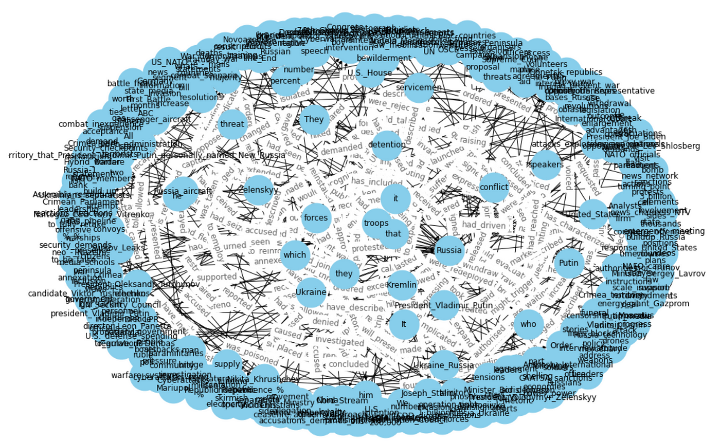
作者提供的图片
知识图谱使我们能够在大局层面上看到所有事物之间的关系,但是像这样很无用...因此最好基于我们正在寻找的信息应用一些过滤器。对于此示例,我将只取涉及最常见实体的图形部分(基本上是最连接的节点):
dtf["entity"].value_counts().head()

作者提供的图片
## filter
f = "Russia"
tmp = dtf[(dtf["entity"]==f) | (dtf["object"]==f)]

## create small graph
G = nx.from_pandas_edgelist(tmp, source="entity", target="object",
                            edge_attr="relation",
                            create_using=nx.DiGraph())

## plot
plt.figure(figsize=(15,10))

pos = nx.nx_agraph.graphviz_layout(G, prog="neato")
node_color = ["red" if node==f else "skyblue" for node in G.nodes]
edge_color = ["red" if edge[0]==f else "black" for edge in G.edges]

nx.draw(G, pos=pos, with_labels=True, node_color=node_color,
        edge_color=edge_color, cmap=plt.cm.Dark2,
        node_size=2000, node_shape="o", connectionstyle='arc3,rad=0.1')

nx.draw_networkx_edge_labels(G, pos=pos, label_pos=0.5,
                        edge_labels=nx.get_edge_attributes(G,'relation'),
                        font_size=12, font_color='black', alpha=0.6)
plt.show()
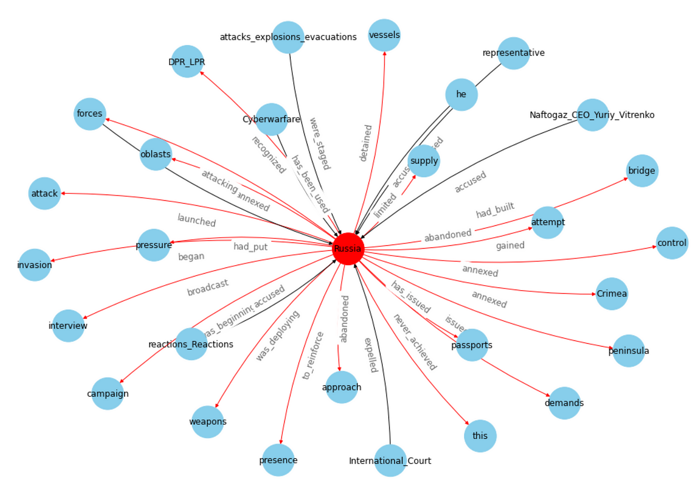
作者提供的图片
这样就好多了。如果你想将其制作成3D,可以使用以下代码:
from mpl_toolkits.mplot3d import Axes3D

fig = plt.figure(figsize=(15,10))
ax = fig.add_subplot(111, projection="3d")
pos = nx.spring_layout(G, k=2.5, dim=3)

nodes = np.array([pos[v] for v in sorted(G) if v!=f])
center_node = np.array([pos[v] for v in sorted(G) if v==f])

edges = np.array([(pos[u],pos[v]) for u,v in G.edges() if v!=f])
center_edges = np.array([(pos[u],pos[v]) for u,v in G.edges() if v==f])

ax.scatter(*nodes.T, s=200, ec="w", c="skyblue", alpha=0.5)
ax.scatter(*center_node.T, s=200, c="red", alpha=0.5)

for link in edges:
    ax.plot(*link.T, color="grey", lw=0.5)
for link in center_edges:
    ax.plot(*link.T, color="red", lw=0.5)

for v in sorted(G):
    ax.text(*pos[v].T, s=v)
for u,v in G.edges():
    attr = nx.get_edge_attributes(G, "relation")[(u,v)]
    ax.text(*((pos[u]+pos[v])/2).T, s=attr)

ax.set(xlabel=None, ylabel=None, zlabel=None,
       xticklabels=[], yticklabels=[], zticklabels=[])
ax.grid(False)
for dim in (ax.xaxis, ax.yaxis, ax.zaxis):
    dim.set_ticks([])
plt.show()
作者提供的图片
请注意,图形可能很有用且好看,但它不是本教程的重点。知识图谱最重要的部分是“知识”(文本处理),然后可以在数据框、图形或不同的绘图中显示结果。例如,我可以使用NER识别的日期构建时间轴图形。
时间轴图形
首先,我必须将被识别为“日期”的字符串转换为datetime格式。DateParser库解析几乎在网页上常见的任何字符串格式的日期。
def utils_parsetime(txt):
    x = re.match(r'.*([1-3][0-9]{3})', txt) #<--check if there is a year
    if x is not None:
        try:
            dt = dateparser.parse(txt)
        except:
            dt = np.nan
    else:
        dt = np.nan
    return dt
让我们将其应用于属性的数据框:
dtf_att["dt"] = dtf_att["date"].apply(lambda x: utils_parsetime(x))

## example
dtf_att[dtf_att["id"]==i]

作者提供的图片
现在,我将其与实体-关系的主要数据框连接起来:
tmp = dtf.copy()
tmp["y"] = tmp["entity"]+" "+tmp["relation"]+" "+tmp["object"]

dtf_att = dtf_att.merge(tmp[["id","y"]], how="left", on="id")
dtf_att = dtf_att[~dtf_att["y"].isna()].sort_values("dt",
                 ascending=True).drop_duplicates("y", keep='first')
dtf_att.head()
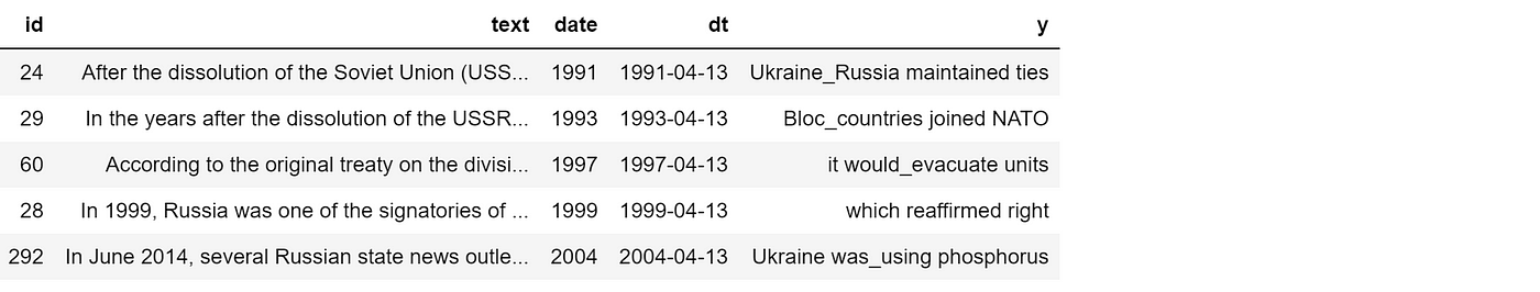
作者提供的图片
最后,我可以绘制时间轴。正如我们已经知道的那样,完整的绘图可能不会很有用:
dates = dtf_att["dt"].values
names = dtf_att["y"].values
l = [10,-10, 8,-8, 6,-6, 4,-4, 2,-2]
levels = np.tile(l, int(np.ceil(len(dates)/len(l))))[:len(dates)]

fig, ax = plt.subplots(figsize=(20,10))
ax.set(title=topic, yticks=[], yticklabels=[])

ax.vlines(dates, ymin=0, ymax=levels, color="tab:red")
ax.plot(dates, np.zeros_like(dates), "-o", color="k", markerfacecolor="w")

for d,l,r in zip(dates,levels,names):
    ax.annotate(r, xy=(d,l), xytext=(-3, np.sign(l)*3),
                textcoords="offset points",
                horizontalalignment="center",
                verticalalignment="bottom" if l>0 else "top")

plt.xticks(rotation=90)
plt.show()
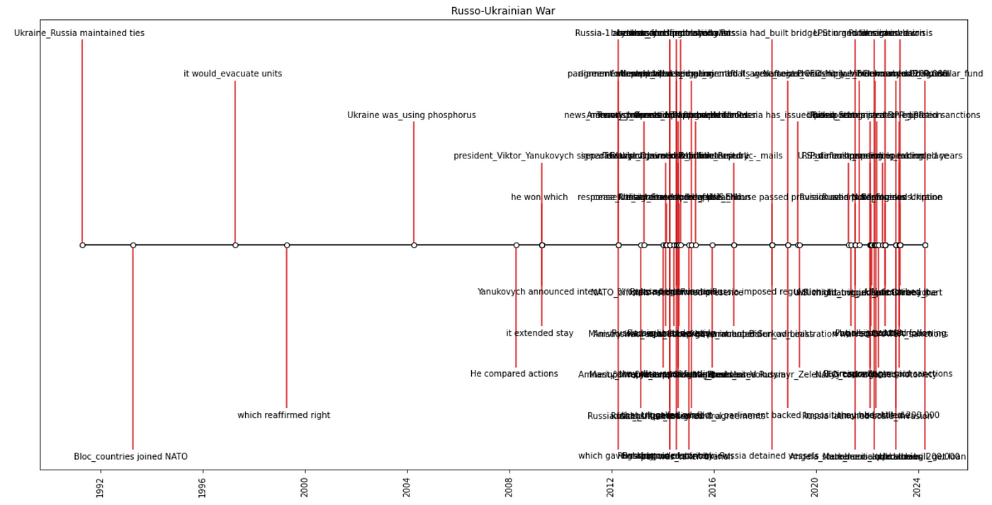
作者提供的图片
因此,最好过滤特定的时间:
yyyy = "2022"
dates = dtf_att[dtf_att["dt"]>yyyy]["dt"].values
names = dtf_att[dtf_att["dt"]>yyyy]["y"].values
l = [10,-10, 8,-8, 6,-6, 4,-4, 2,-2]
levels = np.tile(l, int(np.ceil(len(dates)/len(l))))[:len(dates)]

fig, ax = plt.subplots(figsize=(20,10))
ax.set(title=topic, yticks=[], yticklabels=[])

ax.vlines(dates, ymin=0, ymax=levels, color="tab:red")
ax.plot(dates, np.zeros_like(dates), "-o", color="k", markerfacecolor="w")

for d,l,r in zip(dates,levels,names):
    ax.annotate(r, xy=(d,l), xytext=(-3, np.sign(l)*3),
                textcoords="offset points",
                horizontalalignment="center",
                verticalalignment="bottom" if l>0 else "top")

plt.xticks(rotation=90)
plt.show()

作者提供的图片
正如你所看到的,一旦提取了“知识”,你可以以任何你喜欢的方式绘制它。
结论
本文是一篇关于如何使用Python构建知识图谱的教程。我在从维基百科解析的数据上使用了几种NLP技术来提取“知识”(即实体和关系),并将其存储在网络图对象中。现在你明白了为什么公司正在利用NLP和知识图谱来从多个来源映射相关数据并找到对业务有用的见解。想象一下,如果将这种模型应用于与单个实体(例如苹果公司)相关的所有文档(即财务报告、新闻、推文),可以提取多少价值。你可以快速了解与该实体直接连接的所有事实、人员和公司。然后,通过扩展网络,甚至可以获取与起始实体(A->B->C)没有直接关联的信息。
译自:https://towardsdatascience.com/nlp-with-python-knowledge-graph-12b93146a458


评论(0)